Three ways to track Greenplum queries that use too much resources

Contents

Method 1. Apply EXPLAIN ANALYZE to a query
Method 2. Use system views
- The gp_toolkit schema
- The gp_internal_tools extension
Method 3. Track process metrics

Hello! My name is Roman. I work as a developer at Arenadata, where we meet a lot of challenges related to Greenplum. Once I had the opportunity to deal with a difficult but quite typical case for this DBMS. It was necessary to find out which queries required an inappropriate amount of system resources to be processed. In this article, I would like to share my experience and talk about three methods I have tested to monitor the utilization of system resources consumed by Greenplum queries.

Method 1. Apply EXPLAIN ANALYZE to a query

The first method you can use is to run a query with EXPLAIN ANALYZE and parse the query plan. It allows you to get a variety of information on memory, for example:

Amount of memory allocated for the query.
Number of slices completed. A slice is an independent part of the plan. It can be executed both in parallel and sequentially with other parts. Each slice can consist of several operators.
Amount of memory allocated for each slice and other parameters.

If you enable additional configuration parameters, such as explain_memory_verbosity and gp_enable_explain_allstat, and run EXPLAIN (ANALYZE, VERBOSE) instead of EXPLAIN ANALYZE, you can get even more data about the memory state:

How much memory was required to execute all slices and each slice separately.
How much memory was used to execute the query for each slice.
Information on memory in the context of operations within the query.
Detailed information on memory usage for each segment and other parameters.

For those who have a strong spirit, you can also try EXPLAIN (ANALYZE, VERBOSE) SELECT on a small table with the explain_memory_verbosity and gp_enable_explain_allstat parameters enabled. The output of the command should be a query plan detailing the operations that the segments performed when executing this query, with extended memory information. It is quite difficult to understand such plan — the difficulty lies in the fact that this plan can only be obtained after the query completion. What if the query fails because of memory? Or you need to look at the current memory consumption? Or you need information on other metrics? Alas, EXPLAIN ANALYZE is not helpful in these cases.

Method 2. Use system views

There are several system views that you can use to analyze consumed resources (such as memory and CPU).

The gp_toolkit schema

If the resource group mechanism is used for resource control, then any query that runs inside Greenplum always runs within a specific resource group. The choice of resource group depends on a user who launched the query, since users are associated with a specific resource group. Information about whether a query belongs to a specific resource group can be found in the rsgname field of the pg_stat_activity system view. If you need to understand which resource group a user is assigned to, you can use the following query:

SELECT rolname, rsgname FROM pg_roles, pg_resgroup WHERE pg_roles.rolresgroup = pg_resgroup.oid;

Greenplum from Arenadata uses the resource group mechanism by default. Vanilla Greenplum uses resource queues by default.

When using the resource group mechanism to monitor memory and CPU, you can use views from the gp_toolkit schema:

Views from the gp_toolkit schema

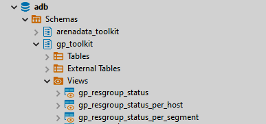
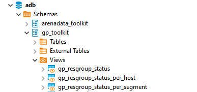
In Greenplum 5 and Greenplum 6, these views are implemented differently, so I’ll tell you about each one separately.

Greenplum 5 (GP5)

In GP5, the only one gp_toolkit.gp_resgroup_status view with the cpu_usage and memory_usage fields is available. The data is presented in JSON format and shows resource utilization in the corresponding resource groups for each segment.

There is a small feature of displaying CPU utilization — if segments are located on the same segment host, they will show the same CPU value (utilization of the segment host on which these segments are located).

The cpu_usage field shows the current CPU utilization:

{"-1":0.02, "0":86.96, "1":87.14, "2":87.15, "3":87.10}

The memory_usage field shows the current memory utilization:

{"-1":{"used":11, "available":2534, "quota_used":508, "quota_available":0, "quota_granted":508, "quota_proposed":508, "shared_used":0, "shared_available":2037, "shared_granted":2037, "shared_proposed":2037},
  "0":{"used":164, "available":472, "quota_used":126, "quota_available":0, "quota_granted":126, "quota_proposed":126, "shared_used":38, "shared_available":472, "shared_granted":510, "shared_proposed":510},
  "1":{"used":0, "available":636, "quota_used":126, "quota_available":0, "quota_granted":126, "quota_proposed":126, "shared_used":0, "shared_available":510, "shared_granted":510, "shared_proposed":510},
  "2":{"used":171, "available":465, "quota_used":126, "quota_available":0, "quota_granted":126, "quota_proposed":126, "shared_used":45, "shared_available":465, "shared_granted":510, "shared_proposed":510},
  "3":{"used":0, "available":636, "quota_used":126, "quota_available":0, "quota_granted":126, "quota_proposed":126, "shared_used":0, "shared_available":510, "shared_granted":510, "shared_proposed":510}
}

The memory_usage field has a more complex structure, so I describe keys of this field (all values are in megabytes):

used — amount of memory used by the query (quota_used + shared_used).
available — amount of memory available for the resource group (quota_available + shared_available). A value can be negative if the query has gone beyond the resource group memory consumption and started consuming global memory.
quota_used — amount of fixed memory used.
quota_available — amount of free fixed memory.
quota_granted — amount of fixed memory that is allocated for the resource group by the memory_limit parameter (quota_used + quota_available).
shared_used — amount of shared memory used.
shared_available — amount of free shared memory. This value can also be negative if the query has gone beyond the resource group memory consumption and started consuming global memory.
shared_granted — amount of shared memory that is allocated for the resource group by the memory_shared_quota parameter (shared_used + shared_available).

Greenplum 6 (GP 6)

In GP6, there are two more views in addition to gp_resgroup_status:

gp_resgroup_status_per_segment
gp_resgroup_status_per_host

They work over the gp_resgroup_status view and provide data on used resources both in terms of segments (gp_resgroup_status_per_segment) and in terms of segment hosts (gp_resgroup_status_per_segment).

It is worth noting that there are a number of limitations in working with these views. Firstly, they show data online only, and unfortunately there is no way to view historical data. Secondly, it is impossible to segment resource consumption within a session and within queries. Since multiple queries from different users can run simultaneously in a resource group, there is no way to understand which query is using which part of the resources.

The gp_internal_tools extension

There is one more interesting view that allows you to control memory resources within a session. It does not depend on whether you use resource queues or resource groups as resource control. The view is in the gp_internal_tools extension and is called session_state.session_level_memory_consumption. To use it, just install the extension with the CREATE EXTENSION gp_internal_tools command. A detailed description of this view fields can be found in Greenplum documentation.

The result of running a query to this view will look something like the image below.

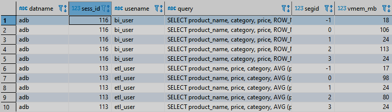
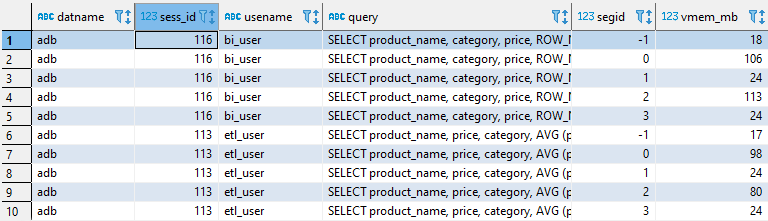
The result of the query to gp_internal_tools

The result of the query against gp_internal_tools

For memory monitoring, we are most interested in the vmem_mb field. It displays how much memory queries are using within a particular session. Using this view, you can detect queries run within a specific session and understand how much memory is consumed within a session.

The sess_id field is the number of the session within which a query is executed. You can use it to combine with the pg_stat_activity system view and get more information on the current query. Since the data is presented for each segment, memory consumption can be tracked by segments. Thanks to this, you can see imbalances in the use of memory when executing queries, if any.

Like the resource group views mentioned above, this view shows data at the time of running a query only, i.e. no historical data is available. If it is needed for subsequent analysis of query execution, you can save data to an internal table. For this:

Create an internal table.
Add a column with the time of data insertion to the table.
Using a task scheduler (for example, cron), run SELECT + INSERT against the session_state.session_level_memory_consumption view into the internal table.

This approach allows you to dynamically track which queries were running in the system and how much memory was allocated for their execution.

This view has the following feature: for the same session, it can display data for the same segment several times (depending on the specific query). It is noteworthy that this does not mean that this query consumes as many times more memory, but you should just keep this in mind.

Method 3. Track process metrics

The third way (and the most interesting, as I see it) is to track metrics of the query processes in the operating system. Each query that starts inside Greenplum generates processes on the master server and segment hosts. It is worth noting that there can be quite a lot of these processes, and their number depends on the complexity of the query and the number of segments on a segment host.

Such processes have certain markers in the launch arguments, which can be used to identify the session number, segment number, query number within the session, and even slice number.

For example, when you run SELECT * FROM <table_name>, pay attention to the processes of the master server and segment host during this query execution — you will see something like the following process on the master:

gpadmin  15322  0.3  0.5 645872 47192 ? Ssl  07:49   0:00 postgres:  5432, gpadmin adb [local] con9 cmd8 SELECT

On the segment server, the same query will generate the following processes:

gpadmin  12020  2.4  0.5 870812 40096 ? Dsl  07:50   0:00 postgres: 10000, gpadmin adb 10.92.8.40(40642) con9 seg1 cmd9 slice1 MPPEXEC SELECT

gpadmin  12021  2.6  0.5 870892 41404 ? Dsl  07:50   0:00 postgres: 10001, gpadmin adb 10.92.8.40(54924) con9 seg3 cmd9 slice1 MPPEXEC SELECT

In this monitoring method, it is also important to understand the meaning of the arguments for launching processes on the master server and segment host. I’ll tell you briefly about them.

Session number. We are talking about the con9 parameter. It is responsible for the session number within which the query runs. Using this number, you can link all processes on the master server and segment hosts that are generated by queries running within this session. And the same session number is present in the sess_id field of the pg_stat_activity system view, from where you can get additional information about the query.
Segment identifier. The process arguments also contain the segment number. In the example above, it is represented as the seg3 and seg1 parameters on the segment hosts. It may be absent in a process on the master server, but there is always one segment on the master server, and its number is -1. The segment number is important if you need to obtain the inequality of resource consumption by different segments.
Command number. There is also the cmd parameter (command count), which is responsible for the command number within a given session. Within one query, it can differ on the master server and on segments. Moreover, even within the same query, cmd can be different on the same segment. For example, this happens when we use a function, and there is a set of commands and queries that are executed within the scope of that function. Thus, it turns out that when executing a certain function, each command inside it will have a different command count, but it will look like one query from the user’s point of view.
Slice number. You can also get the slice number from the process arguments. In the above example, the slice is represented by the slice1 parameter on the segment hosts. On the master server, the slice is not mentioned in the process arguments. However, in some cases this parameter may also be present in the process on the master server. This means that this part of the query was executed directly on the master server. This way we can get data on the query being executed in the context of slices and see which slice requires the most memory or uses the most CPU.

Once we have figured out the arguments of processes, next is a matter of technique. For each process, we collect the necessary metrics, aggregate data from all segments by a session number (con in process arguments and sess_id in the pg_stat_activity system view), and get metrics for a query that was executed in Greenplum within a certain session at the time of collecting metrics.

Collection and aggregation is a creative process. For example, you can use popular monitoring systems, which include monitoring agents that can collect the necessary metrics for processes and a centralized database where data can be aggregated. You can also use your own scripts and your own database.

Which process metrics can be collected?
CPU utilization

There are some nuances here. For example, the ps utility shows the average value since the process appeared in the system. This is not very convenient when you need to track peak loads at a certain point in time. Let’s say a query worked on some slice for a long time and did not require special resources, but at some point in time the slice has worked, and another slice requiring large CPU resources came into play. In this case, the average CPU usage will be small, since the process of this slice has not performed any active actions until the current moment.

Therefore, it is better to monitor the current CPU load and, based on this data, calculate the average value over a certain period of time if necessary.

Current CPU utilization can be obtained via the top or htop utilities. You can use data from the /proc/uptime and /proc/[pid]/stat files. If you use data from files, the calculation algorithm will be the following:

Get the number of ticks per second (clk_tck) using the getconf CLK_TCK command.
Get the uptime time (cputime) using the first parameter of the /proc/uptime file.
Get the total time (proctime) spent by the process (utime(14) + stime(15)) from /proc/[pid]/stat.
Wait 1 second and repeat steps 2 and 3.
Calculate the percentage of CPU usage using the formula:

Load on the disk subsystem

There are also a number of utilities here that display data by processes (for example, iotop or pidstat), or you can get data from the /proc/[pid]/io process file.

It is important to understand that this is only a part of the load on the disk subsystem that is generated by this particular process. Don’t forget about background service processes that synchronize data between the main segment and its mirror, write data to the transaction log, and so on. Depending on the query type, these service processes may generate additional load on the disk subsystem.

Memory

This is the most interesting metric. Let me remind you that there are two main system views in Greenplum that show data on memory:

The session_state.session_level_memory_consumption view (the vmem_mb field), which shows the total amount of memory used within a session.
Resource group view, which displays data on memory (used by queries running within a specific resource group).

Depending on the query complexity, the data on memory in these system views can vary significantly. This is due to some subtleties of accounting for the memory provided to the process, for which the internal Greenplum mechanism is responsible. Typically, the numbers in the session_level_memory_consumption view are larger than those in the resource group view.

This is actually not so critical, since there is a correlation between values in two views.

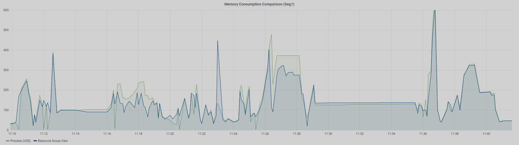
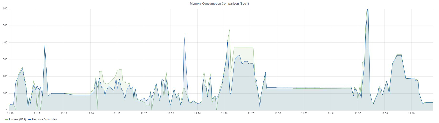
Below are graphs of memory consumption from two views for 97 queries with a small amount of data from the standard TPC-DS test.

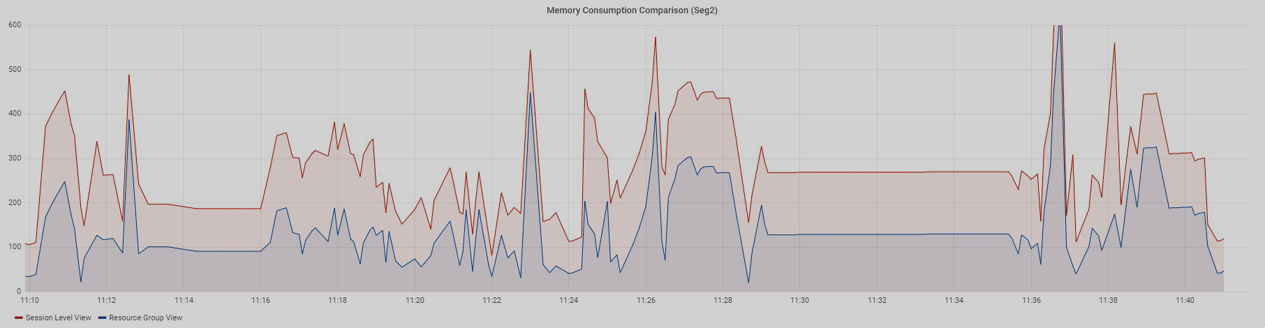
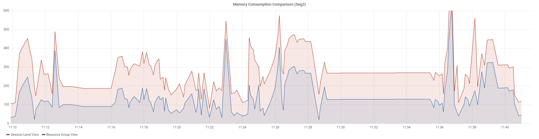
Graph comparing memory consumption data between Resource Group View and Session Level View

Queries were executed sequentially.

The Resource Group View graph is built using data from the memory_used column of the gp_toolkit.gp_resgroup_status_per_segment view, and the Session Level View graph is built based on data from the vmem_mb column of the session_state.session_level_memory_consumption view.

Both graphs display data for one segment. The graphs show that if memory consumption in a resource group increases, the value from the session_level_memory_consumption view increases too, and vice versa.

Thus, using the session_level_memory_consumption view, you can track the trend of memory consumption by a query running within a specific session.

But let’s return to our processes, which are generated by queries inside Greenplum. Let’s try to find out how much memory is consumed by processes and compare the resulting numbers with memory from system views.

Using the ps -eo pid, rss, command commands, we can get data about the RAM allocated for the process — Resident Set Size.

The calculation algorithm is the following:

Get PID of all processes on the master server and segment hosts that relate to queries. Just above I have already shown how these processes look like. Exclude processes that have passed into the idle state (if a process has passed into the idle state, this means that this process has already completed or is waiting).
Obtain data on Resident Set Size for each process.
Sum up values received from processes and group them by session_id (cmd in the process arguments) and seg_id (the seg value in the process arguments). We get the result presented on the graph.

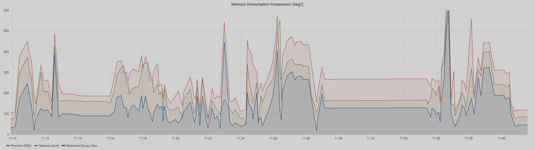
Graph comparing memory consumption data between Resource Group View and Session Level View + data on RSS memory from processes

The Process (RSS) graph, which displays the sum of RSS across all processes of a particular query, is somewhere in the middle between the Session Level View and Resource Group View graphs and follows the trend of two accompanying graphs.

In addition to Resident Set Size, processes have 2 more types of memory — Unique Set Size and Proportional Set Size. The results of the experiments showed that if we need to get closer to the data displayed in the resource group view, Unique Set Size is the closest to this value.

We use the same calculation algorithm as when using data on RSS, but now we need data on USS memory. You can use the smem utility or get data from the /proc/[pid]/smaps file. When using the smaps file, you can obtain the USS value by summing all the values for the Private_Clean and Private_Dirty fields. The value will be in kilobytes.

If we perform all operations of the algorithm, we will get a value close to the memory_used value from the gp_resgroup_status_per_segment view obtained at the same point in time.

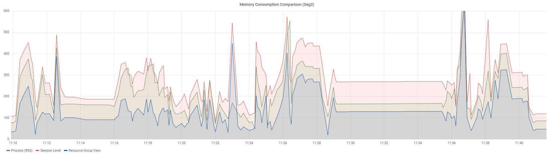
Below are graphs of the same 97 queries for two segments: Seg1 and Seg2.

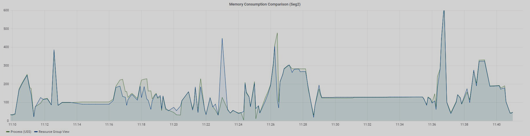
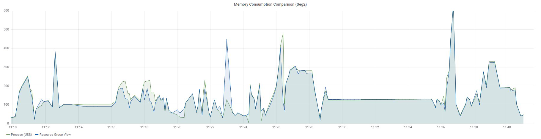
Graph comparing memory consumption data between Resource Group View and USS memory data from processes (Seg1)

Graph comparing memory consumption data between Resource Group View and USS memory data from processes (Seg2)

Queries were executed sequentially — at a particular time, only one query was running in the measured resource group. Let me remind you that there is no way to divide memory usage for each query in resource group views. You can only see the overall value for all queries running in a specific resource group.

The Resource Group View graph displays data from the gp_resgroup_status_per_segment view by values in the memory_used column, and the Process (USS) graph shows the sum of USS for all processes of a particular query.

There is also no clear match, but the values are very close, especially for Seg2. Why do I say "close"? The fact is that Greenplum has its own internal mechanism for accounting virtual memory — vmtracker. It is responsible for how much memory to allocate to a query, how much memory is left free, whether it is possible to allocate additional memory to a query, or whether there is no free memory. How this virtual memory relates to the memory consumed by the query processes is a matter for a separate study that I have yet to figure out someday. The results I have described were obtained experimentally.

Of course, you may have a reasonable question: why do we need metrics from processes if we have system views and don’t have to bother collecting, aggregating, and storing these metrics?

I will answer the following.

Firstly, if we use data from resource group views, we can select a specific query in this group only if it works alone within this resource group. If there are two or more processes running in parallel, it is impossible to separate these resources.

Secondly, this makes it possible to see resource consumption by slices. We can find out memory consumption almost at the level of operators inside slices. You can see which operators are executed inside a slice using the EXPLAIN command. This command will display the query execution plan, but will not physically execute the query.

Thirdly, you can collect any process metrics that are necessary for statistics, but which are not in system views.

This is probably all I wanted to tell you about the system metrics that can be collected and monitored within the scope of query work in Greenplum.

Found a mistake? Seleсt text and press Ctrl+Enter to report it